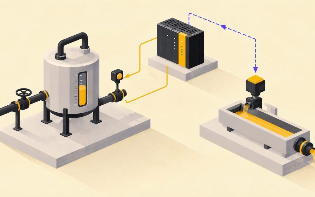
A control system measures what a machine or process is doing, compares it with what you want, and acts to close the gap. Learn that loop (reference, error, controller, actuator, plant, sensor) and you can read almost any control diagram and most PLC programs. This guide covers the fundamentals, then shows how they apply to PLC programming and troubleshooting on a plant floor. We teach this at Online PLC Support, where the theory is tied to real controllers from the first lesson.
TL;DR
- A control system commands, directs, or regulates a physical process so its real state matches the state you want.
- Every loop has the same parts: setpoint, comparator, controller, actuator, plant, and sensor (plus a feedback path in closed-loop designs).
- Open-loop control acts without checking the result. Closed-loop control measures the result and corrects for disturbances.
- Judge any loop by stability, steady-state error, and transient response: overshoot, rise time, peak time, and settling time.
- In a PLC, the controller is your program, the sensors are your inputs, and the actuators are your outputs. Troubleshooting is walking the loop one element at a time.
Table of Contents
- What a control system is
- The basic elements of a control loop
- Open-loop vs. closed-loop control
- Reading a block diagram
- How to judge whether a loop performs well
- Types of control systems you will meet
- Applying the fundamentals to PLC programming
- Using the loop to troubleshoot
- A study path that builds on the basics
- Our perspective
- Put the fundamentals to work with us
- FAQ
- Sources
What a control system is
A control system is a collection of mechanical and electrical devices connected to command, direct, or regulate a physical plant. Its goal is to drive the plant’s real state variables to equal the desired state variables. In control language, the “plant” is simply the thing being controlled: a tank, a conveyor, a furnace, a motor.
That definition is deliberately broad. A home thermostat, a car’s cruise control, a bottling line, and a robot arm all fit it. What changes from one to the next is how fast the plant reacts, how much the environment pushes back, and how precisely you need the output held.
For an industrial technician the practical meaning is this: somebody wants a number to be a particular value (a temperature, a speed, a position, a pressure, a level), and the control system keeps it there while the world tries to push it away.
The basic elements of a control loop
Textbooks name slightly different blocks, but the set is stable. A standard treatment lists the reference or setpoint, comparator, controller, actuator, plant, sensor, and the feedback path where feedback is used. Here is each element in plain terms, with a heated-tank example.
| Element | What it does | Heated-tank example |
|---|---|---|
| Reference (setpoint) | The value you want | 150°F |
| Comparator | Subtracts the measurement from the reference to form the error | Setpoint minus measured temperature |
| Controller | Computes an action from the error | The PLC program or a PID instruction |
| Actuator | Applies the action to the plant | Steam valve or heater contactor |
| Plant | The process being controlled | The tank and its liquid |
| Sensor | Measures the controlled quantity | RTD or thermocouple with a transmitter |
The University of Illinois ECE 486 handbook describes the same roles: the plant is the system being controlled, sensors measure the controlled quantity, actuators act on the plant, and the controller processes sensor signals to drive the actuators. Its companion notes also name reference, error, disturbances, and control input as the standard variables around those blocks.
Disturbances are the part newcomers skip. They are anything that pushes the plant away from the setpoint without being asked: cold water entering the tank, a heavier load on a motor, a door left open. Control exists because of disturbances. If nothing ever changed, you would set the actuator once and walk away.
Open-loop vs. closed-loop control
This is the most important distinction in the subject, and it decides how a machine behaves when something goes wrong.
Open-loop control sends a command and never checks the result. An open-loop system has no state estimator or feedback path and can have large errors. The same source lists examples such as a toaster, a timed irrigation sprinkler, and stepper motors. They run on a timer or a fixed command, so they have poor sensitivity to disturbances: if it rains, the sprinkler still runs.
Closed-loop control measures the output and feeds it back. A closed-loop system uses the measurement in feedback to drive errors toward zero. Berkeley’s feedback control lecture notes that closed-loop systems gather measurements, feed them back, and compare them, which is why they can correct for disturbances while open-loop systems cannot compensate for them. Cruise control is the classic case. A thermostat controlling a furnace is another.
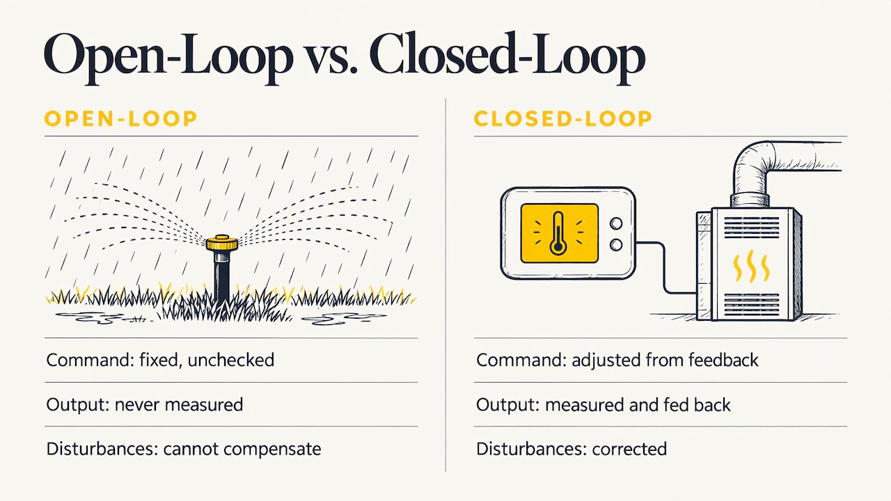
Control Engineering describes the closed-loop sequence as a repeating chain of process, sensor, transmitter, controller, and actuator, continuing until the desired process condition is reached.
Which one do you see in a plant?
Both. A conveyor that runs for a fixed time after a start button is open-loop. A conveyor whose speed is held by a drive reading encoder feedback is closed-loop. Many machines mix the two: discrete sequencing (do this, then that) wrapped around a few closed loops for temperature, pressure, flow, or speed. Recognizing which part of a machine is which is the first skill in reading an unfamiliar system.
Reading a block diagram
Block diagrams are the shorthand language of control. A block represents a functional relationship, and arrows carry signals between blocks. Each block has an input and an output, and a summing junction adds or subtracts signals. That summing junction is the comparator from the table above.
Three reading rules save a lot of confusion:
- Follow the arrows, not wires. A guide from IEEE warns that block diagrams help analyze feedback and should not be confused with circuit diagrams, because the connecting lines are not wires.
- Find the error first. The relation is e = r − y: the error is the reference minus the measured output, as shown in MATLAB’s documentation. If you can locate that subtraction, you have found the heart of the loop.
- Label the signals. MIT’s introductory handout uses open-loop and closed-loop block diagrams to identify the system input, output, error, and control signal, and calls the diagrams critical for analyzing control logic. Do the same on any machine you inherit.
A useful exercise: take a machine you know, draw the six blocks, and write the real device name in each one. Gaps in the drawing, such as “I don’t know what actually measures this,” are usually the same gaps that make troubleshooting slow.
How to judge whether a loop performs well
A loop that eventually reaches the setpoint is not necessarily a good loop. The performance questions are consistent across textbooks. The University of Texas guide says effectiveness is commonly evaluated using steady-state controller error, stability, and transient response. MIT frames the same ideas as stability, steady-state error, convergence rate, and noise rejection.
Stability
Berkeley’s lecture characterizes a stable natural response as one that decays to zero, a sustained oscillation as one that holds system energy, and an unstable response as one that grows without bound. On the floor, instability looks like a valve hunting back and forth, a motor surging, or a temperature that swings wider with every cycle.
Transient and steady-state response
Rutgers’ engineering notes define the transient response as the initial response after startup and the steady-state response as the long-run component left after transient behavior decays. The listed transient metrics are overshoot, settling time, peak time, and rise time.
| Metric | Plain meaning | What it looks like on a machine |
|---|---|---|
| Rise time | How fast the output first approaches the setpoint | How quickly a tank heats up after a setpoint change |
| Overshoot | How far past the setpoint it goes | Temperature spikes above the target before settling |
| Peak time | When the highest point occurs | When the spike tops out |
| Settling time | How long until it stays near the setpoint | When operators can trust the reading |
| Steady-state error | The leftover gap once things settle | A tank that parks at 147°F instead of 150°F |
The University of Texas chapter adds that you should watch for oscillations, rapid changes, and high output magnitudes. Those three symptoms are exactly what an operator reports as “it’s acting weird.”
Types of control systems you will meet
Control systems are classified several ways. Common classifications include continuous, SISO (single input, single output), MIMO (multiple input, multiple output), open-loop, and closed-loop systems, with robots as a typical MIMO example. Inside closed-loop designs, the most common controller you will touch is PID, and the University of Texas guide covers PI and PID controllers.
In industry, the hardware that runs these loops falls into a few families. Control Engineering identifies PLCs and PACs as industrial computers that control production systems, and lists DCS and SCADA among control-system types. A rough guide to where each fits:
- PLC: discrete machine control, sequencing, interlocks, and many small loops. If you want to see how the hardware differs by size and purpose, our overview of types of PLCs is a good next read.
- DCS: large continuous processes where many loops are managed together.
- SCADA: supervisory visibility and data collection across a site or many sites.
Applying the fundamentals to PLC programming
This is where theory turns into paychecks. Map the loop onto a PLC and every element has a home.
| Control element | Where it lives in a PLC system |
|---|---|
| Sensor | Input module: photoeyes, proximity switches, pressure and temperature transmitters |
| Comparator and controller | Your program: comparison instructions, PID instruction, ladder rungs |
| Actuator | Output module or drive: contactors, solenoids, VFDs, servo drives |
| Plant | The machine or process |
| Reference | Operator setpoint on an HMI screen or a stored recipe value |
A PLC repeats a cycle: it reads inputs, executes the program, writes outputs, and handles communications and diagnostics. That repeating cycle is the digital version of the measure-decide-actuate loop. Two practical consequences follow. First, a PLC only knows what its input image says at the moment it reads, so a very fast pulse can be missed. Second, the order of rungs matters, because the program is solved in sequence.
Discrete logic is control too
Ladder logic that starts a motor when a start button is pressed and no stop or overload is active is open-loop in the strict sense: it issues a command without measuring the outcome. Add a run-feedback contact or a no-motion timer that faults the motor if the feedback never arrives, and you have closed a loop. That small pattern, command plus confirmation plus fault, appears on nearly every well-built machine. You can see how instructions are put to work in our walkthrough of PLC instructions in use.
Analog loops and PID
When the quantity is continuous, such as temperature, flow, or level, the PLC typically runs a PID loop. The vocabulary from the previous section tells you what to tune for: faster rise time costs overshoot, and aggressive action can cost stability. Setpoint, process variable, and control output on a PID instruction are the reference, sensor measurement, and actuator command from the block diagram. For more on how these ideas show up in code, see our page on PLC programming controls.
Using the loop to troubleshoot
The fundamentals give you a fixed route for any fault: walk the loop. A step-by-step approach to a misbehaving actuator follows the same order, checking the power supply, sensors, mechanical components, feedback loop, and performance. Here is the version we would hand a maintenance technician:
- Confirm the reference. Is the setpoint what you think it is? Check the HMI value and the value in the controller, because they can differ.
- Check the sensor. Does the live input value match reality? Dirt, moisture, damage, and calibration errors are common causes of bad readings. A wrong measurement makes the controller correct toward the wrong target.
- Look at the error. Compare setpoint and process variable in the online program. If the error is large and the output is saturated at 100% or 0%, the controller is trying but the plant is not responding.
- Test the controller output. Is the program commanding what it should? Forces, overridden bits, and manual mode on a PID block are frequent culprits.
- Check the actuator. Does the output module energize? Does the valve, drive, or contactor respond? Look for lockouts, tripped drives, and air or hydraulic supply problems.
- Inspect the plant. A stuck valve, slipping belt, or fouled heat exchanger can make a healthy loop look broken.
- Classify the symptom. Oscillation points toward tuning or a sticky actuator. A constant offset points toward steady-state error, which can come from an actuator limit or missing integral action. Slow response points toward a sluggish actuator or conservative tuning.
This is also why drawing the block diagram pays off: each step is a block, and you isolate the failure by elimination instead of guessing.
A study path that builds on the basics
The fundamentals are a short subject. Turning them into skill takes practice on real hardware and real software, in this order:
- Learn to read and draw block diagrams until the six elements are automatic.
- Learn ladder logic and how a controller scans inputs and outputs.
- Work through a PID loop on a real or simulated process, changing one gain at a time and watching overshoot and settling time.
- Practice fault-finding on an application you can break and fix safely.
Our guide to what to learn and how to choose a control systems course lays out this sequence in more detail, and the broader industrial automation training page shows where it leads.
Our perspective
Most people who struggle with PLCs do not struggle with the instructions. They struggle because nobody showed them the loop behind the instructions. Once you see a program as sensor, decision, and actuator, an unfamiliar machine stops being a wall of rungs and becomes a set of questions you can answer in order.
That is why our training is built around real-life examples and hands-on strategies. We teach the fundamentals with the same industry-standard software you will use on the job, such as RSLogix 500, RSLogix 5000, Studio 5000, and FactoryTalk View Studio, so the concept and the screen it lives on are learned together.
We designed our courses to be clear, structured, and cost-effective for every skill level, from a student writing a first rung to an engineer or maintenance professional who needs better troubleshooting technique. We keep the content current, because the people we train deserve methods that match what is on their plant floor today.
the author
Put the fundamentals to work with us
If you want to move from concepts to controllers, our online courses, video tutorials, and how-to articles cover PLC and HMI programming, troubleshooting methods, and the Allen-Bradley software above. Our Allen Bradley PLC training and related courses are the place to start for structured, on-demand learning.
If you would rather work on your own machine or your own questions, we offer one-on-one coaching from $67 per session, and a 90-minute PLC coaching session for $97. A yearly PLC training membership is $192 per year, and you can see the details on our membership and programming services page.
FAQ
What are the basic parts of a control system?
The basic parts are the setpoint, comparator, controller, actuator, plant, and sensor, plus a feedback path in closed-loop systems. The sensor measures the plant, the comparator forms the error, the controller computes an action, and the actuator applies it. In a PLC system these map to input modules, your program, and output modules or drives.
What is the difference between open-loop and closed-loop control?
Open-loop control sends a command without checking the result, so it cannot correct for disturbances. Closed-loop control measures the output, compares it with the setpoint, and corrects the error. A timed sprinkler is open-loop, and a thermostat-controlled furnace is closed-loop.
Do I need advanced math to learn control systems basics?
Not to start. You can understand the loop, read block diagrams, and troubleshoot using the concepts of setpoint, error, overshoot, and settling time without solving equations. The math becomes useful later, if you move into controller design and analysis.
How do control systems fundamentals help with PLC troubleshooting?
They give you a fixed route: check the reference, sensor, error, controller output, actuator, and plant in that order. Each step isolates one block, so you find the failing element by elimination. Symptoms like oscillation or constant offset also point toward likely causes.
Sources
- Chapter 8: Control Systems, University of Texas
- Control Systems Engineering, Cal Poly
- ECE 486 Control Systems handbook, Spring 2026
- ECE 486 Control Systems handbook, Spring 2025
- Open- vs. closed-loop control, Control Engineering
- Feedback Control Systems lecture, Berkeley
- Control Engineering: Basic terms explained
- Control System: Types, Uses, and Components, Thomasnet
- A Student’s Guide to Classical Control, IEEE
- MATLAB connect documentation, MathWorks
- Introduction to Control handout, MIT
- Control: Introduction Mechanical Engineering
- Transient and Steady State Responses, Rutgers